Linear Regression

Linear regression is the first algorithm worth learning deeply because almost every idea in supervised machine learning appears in a simple, inspectable form: features, labels, predictions, loss, optimization, coefficients, residuals, evaluation, assumptions, and failure modes.

The goal is straightforward: predict a continuous number from one or more input features. The number might be house price, salary, demand, temperature, risk, revenue, wait time, or energy usage.

But the deeper lesson is not merely "draw a line." Linear regression teaches how a model becomes a mathematical explanation of a relationship and how to audit whether that explanation deserves trust.

Watch that line form from the residuals, then what one far salary does to the slope.

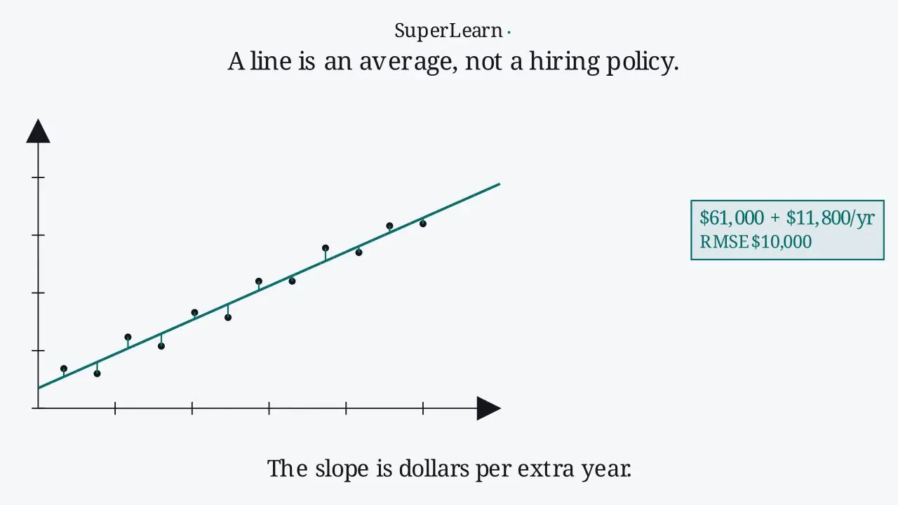
The sections below unpack that salary line, the residual audit, and the least-squares bowl.

The fundamental problem

Suppose you are estimating software developer salaries. You notice that years of experience is related to salary, but not perfectly:

• Two developers with five years of experience may earn different salaries.
• Location, education, company size, specialization, and negotiation all matter.
• Compensation data contains noise, outliers, and local patterns.

Linear regression asks:

What line best summarizes the average relationship between the input feature and the numeric target?

For one feature, the model is:

$$\hat{y} = \beta_0 + \beta_1x$$

Where:

• $\hat{y}$ is the predicted value.
• $x$ is the input feature.
• $\beta_0$ is the intercept, or baseline prediction when $x = 0$.
• $\beta_1$ is the slope, or expected change in prediction for a one-unit increase in $x$.

Here is that equation as a computed still: intercept $61000$ at zero years, slope $11800$ per extra year.

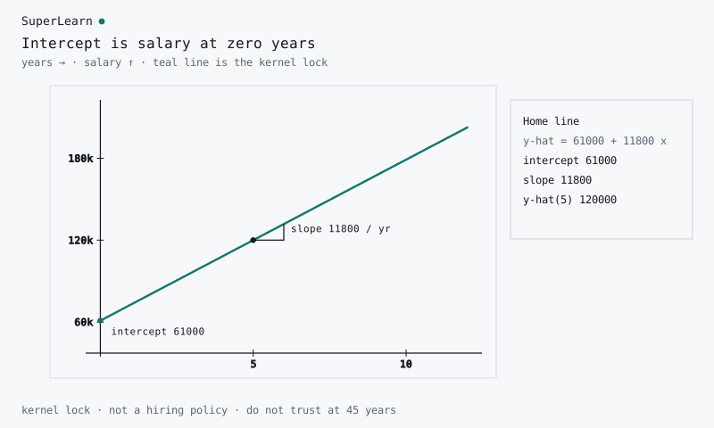
Read intercept and slope from the HUD; they match the kernel lock $61000 + 11800x$.

The intercept is a salary, in dollars, at $x = 0$. The slope is dollars per extra year. Neither number is a hiring policy: the line summarizes an average relationship in the training cloud, and it should not be trusted far outside that cloud.

For multiple features, the same idea becomes:

$$\hat{y} = \beta_0 + \beta_1x_1 + \beta_2x_2 + \cdots + \beta_px_p$$

Linear regression is called "linear" because the prediction is a weighted sum of the features. The original features can still be engineered: a model can include $x^2$, log transforms, interactions, or encoded categories while remaining linear in its coefficients.

Fit the line, then audit the errors

The static diagram below is placed before the math because it establishes the whole workflow in one picture: fit a line, inspect residuals, interpret coefficients, and validate assumptions.

The stems below are ordinary least squares on the lesson home salaries.

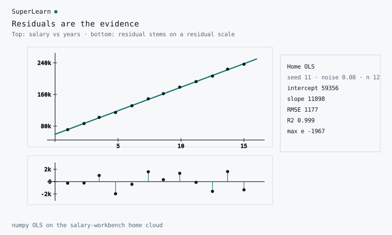
RMSE and $R^2$ in the HUD are numpy on that same fit.

Teal stems are the residuals. If they look like noise around zero, the line captured the average. A U-shape, a funnel, or one long stem at far $x$ is the model telling you the straight-line story is incomplete.

The vertical gaps between points and the line are residuals:

$$e_i = y_i - \hat{y}_i$$

Residuals are not a side detail. They are the evidence. A good linear model should leave residuals that look mostly patternless. If residuals curve, fan outward, cluster by subgroup, or reveal extreme leverage points, the model is telling you that the straight-line story is incomplete.

Least squares: the training objective

Linear regression usually chooses coefficients by minimizing the sum of squared residuals:

$$SSE = \sum_{i=1}^{n}(y_i - \hat{y}_i)^2$$

The average version is mean squared error:

$$MSE = \frac{1}{n}\sum_{i=1}^{n}(y_i - \hat{y}_i)^2$$

Squaring has three important effects:

• Positive and negative errors do not cancel.
• Large errors are penalized more heavily.
• The optimization problem has smooth mathematical structure.

Here is that bowl on the geometry-lab home cloud.

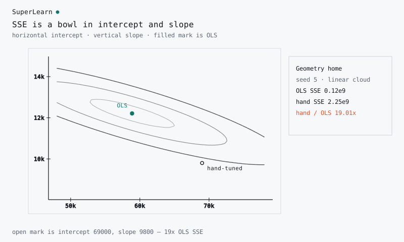
The filled mark is OLS; the open mark is a nearby hand-tuned line with a larger SSE.

Think of every candidate line as a point $(\beta_0, \beta_1)$. Squared error makes a bowl. Ordinary least squares is the unique bottom of that bowl for a linear model. A hand-tuned line can look close and still sit up the wall; a small SSE can still be the wrong story if the cloud itself bends.

The fitted coefficients for ordinary least squares can be written in matrix form:

$$\hat{\beta} = (X^TX)^{-1}X^Ty$$

This is the normal equation. In practice, libraries often use numerically stable decompositions rather than literally computing the inverse, but the formula is still valuable because it shows the central idea: coefficients are chosen from the geometry of the feature matrix and the target vector.

Interact with salary prediction and residuals

Use the workbench here, after the equation and residual idea are clear. Adjust noise, add an outlier, and compare the fitted slope, residuals, RMSE, and $R^2$. The goal is not to memorize a number; it is to feel how the model reacts when the data story changes.

Use the planted-outlier control until the slope stops meaning "typical extra year." A mid-$x$ spike lifts the whole line; a far-$x$ point rotates it. $R^2$ can stay high while the coefficients stop being a story you would publish.

Interpreting coefficients

In a one-feature salary model:

$$\widehat{salary} = 61000 + 11800 \times experience$$

The interpretation is:

• The intercept says the model's baseline is about $61k when experience is zero.
• The slope says each additional year of experience adds about $11.8k to the prediction, holding the model structure fixed.

In multiple regression, "holding other features constant" becomes crucial:

$$\widehat{salary} = \beta_0 + \beta_1 experience + \beta_2 languages + \beta_3 location_sf$$

If $\beta_3 = 30000$, the model estimates a $30k salary premium for San Francisco compared with the reference location, after accounting for the other included features.

This interpretability is a major reason linear regression remains useful. A black-box model might predict slightly better, but a linear model can often explain which factors drive the prediction.

Evaluation metrics

Mean absolute error

$$MAE = \frac{1}{n}\sum_{i=1}^{n}|y_i - \hat{y}_i|$$

MAE is easy to explain: the average absolute miss in the target's units.

Root mean squared error

$$RMSE = \sqrt{\frac{1}{n}\sum_{i=1}^{n}(y_i - \hat{y}_i)^2}$$

RMSE is also in the target's units, but it reacts more strongly to large errors.

R squared

$$R^2 = 1 - \frac{SS_{res}}{SS_{tot}}$$

$R^2$ estimates the fraction of target variation explained by the model. An $R^2$ of 0.82 means the model explains about 82% of the variation in the evaluation data. It does not prove causality, fairness, or production readiness.

Move the line by hand

The salary workbench showed the fitted compromise. The lab below lets you drag intercept and slope yourself. Watch the residual stems and the SSE ratio. Snap back to OLS when you want the unique bottom of the bowl. Then switch the cloud to "slightly curved": OLS still wins on SSE, and the stems still curve.

A small sum of squares is not the same question as "is a straight line the right story." Training walks downhill on this bowl. If the bowl is the wrong shape for the world, the bottom is still the wrong story.

A complete implementation pattern

import pandas as pd
from sklearn.compose import ColumnTransformer
from sklearn.linear_model import LinearRegression
from sklearn.metrics import mean_absolute_error, mean_squared_error, r2_score
from sklearn.model_selection import train_test_split
from sklearn.pipeline import Pipeline
from sklearn.preprocessing import OneHotEncoder, StandardScaler

features = [
    "years_experience",
    "programming_languages",
    "education_level",
    "location",
    "company_size",
]

X = salary_data[features]
y = salary_data["salary"]

X_train, X_test, y_train, y_test = train_test_split(
    X,
    y,
    test_size=0.2,
    random_state=42,
)

preprocess = ColumnTransformer(
    transformers=[
        ("numeric", StandardScaler(), ["years_experience", "programming_languages"]),
        ("categorical", OneHotEncoder(handle_unknown="ignore"), ["education_level", "location", "company_size"]),
    ]
)

model = Pipeline(
    steps=[
        ("preprocess", preprocess),
        ("regression", LinearRegression()),
    ]
)

model.fit(X_train, y_train)
predictions = model.predict(X_test)

mae = mean_absolute_error(y_test, predictions)
rmse = mean_squared_error(y_test, predictions, squared=False)
r2 = r2_score(y_test, predictions)

print({"MAE": mae, "RMSE": rmse, "R2": r2})

The Pipeline matters. It ensures preprocessing is learned from the training split and then applied consistently to test data. That protects against a common leakage mistake: scaling or encoding using the full dataset before splitting.

Diagnostic workflow

A responsible linear regression workflow does not stop after printing $R^2$.

Residuals versus predictions

Plot residuals against fitted values. A random cloud is encouraging. A curve suggests nonlinearity. A funnel shape suggests changing variance.

Residuals versus features

Inspect residuals against each important feature. If the model underpredicts for high experience and overpredicts for low experience, a transformation or interaction may be needed.

Outlier and leverage checks

Some points have unusual target values. Others have unusual feature values. A high-leverage point can tilt the fitted line dramatically. The question is not "delete outliers"; the question is "understand whether this point is valid, rare, influential, and relevant to deployment."

The same home salaries plus one far-$x$ point the workbench can plant.

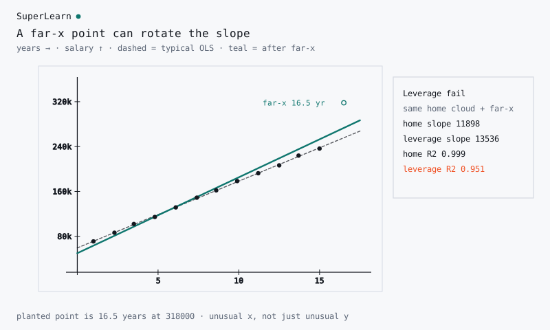
The dashed line is the ordinary fit. The teal line is OLS after one far-$x$ salary is planted. Leverage is unusual $x$, not just an unusual $y$. A spike in the middle lifts the line; a point at the edge of experience can own $\beta_1$.

Subgroup performance

A model can look accurate overall and still fail for a group. Check error by region, seniority level, company size, or any subgroup relevant to the use case.

Assumptions and what they mean

Linear regression is most trustworthy when:

• The relationship is approximately linear after feature engineering.
• Training rows are independent enough for the use case.
• Error variance is reasonably stable.
• Important variables are not omitted in a way that distorts interpretation.
• Features are not perfectly redundant.
• Test data represents the future data distribution.

These assumptions are not bureaucratic fine print. They tell you when coefficient interpretations and uncertainty estimates can be trusted.

Common mistakes

Treating correlation as causation

If experience correlates with salary, that does not mean adding one year of experience mechanically causes the exact coefficient increase. Observational data includes confounding factors.

Extrapolating outside the data range

A line fitted on 0 to 15 years of experience should not be trusted for 45 years of experience without evidence.

Optimizing only training score

A perfect training fit can be a warning sign. Always evaluate on held-out data.

Ignoring the cost of different errors

In salary modeling, underpaying and overpaying may have different business and ethical consequences. In medicine, false negatives and false positives can be radically different.

Extensions

Polynomial features

If the relationship bends, include transformed features:

$$\hat{y} = \beta_0 + \beta_1x + \beta_2x^2$$

The model is still linear in coefficients, but it can represent curves.

Ridge regression

Ridge regression adds an L2 penalty:

$$Loss = SSE + \lambda\sum_j\beta_j^2$$

This shrinks coefficients and can improve generalization when features are correlated.

Lasso regression

Lasso adds an L1 penalty:

$$Loss = SSE + \lambda\sum_j|\beta_j|$$

Lasso can push some coefficients exactly to zero, making it useful for feature selection.

Practical takeaway

Linear regression is useful when you need a fast, interpretable baseline for numeric prediction. It is especially strong when the relationship is roughly linear, the data is well prepared, and the decision-maker needs to understand feature effects.

It is weak when the real pattern is highly nonlinear, interactions dominate, or the cost of errors varies sharply across the input space. Even then, it remains a powerful baseline. If a complex model cannot clearly beat a well-diagnosed linear regression, the simpler model may be the better engineering choice.

Sources consulted

• Google Machine Learning Crash Course for loss, residual intuition, MAE, MSE, RMSE, and outlier behavior.
• scikit-learn documentation for ordinary least squares, linear-model APIs, and pipeline patterns.
• Stanford CS229 notes for supervised-learning notation, least-squares derivation, and normal-equation framing.
• An Introduction to Statistical Learning for model interpretation, diagnostics, and linear regression pedagogy.
• The Elements of Statistical Learning for regularization context and model-selection principles.