Linear Algebra: Leftover Reconstruction, Then Explained Variance

Linear algebra spends leftover reconstruction that a scalar recipe cannot spend. A nearly aligned pair spends leftover on a direction. Leftover orthogonal is what a second axis should spend. Extra unused rank leftover unused rank. Leftover on the true axis remains after the projection. Home still names leftover first, then the pretty explained variance.

The key question is:

After the projection, what leftover reconstruction remains, and did leftover orthogonal sit idle because rank was one or leftover unused rank sit idle because the second axis was extra?

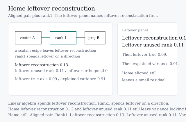
Home still in the lab below is leftover reconstruction: leftover reconstruction 0.13, leftover unused rank 0.11, leftover orthogonal 0, leftover on true axis 0.09. Explained variance still looks fine at 0.91.

A scalar recipe treats knowledge as leftover already spent as one number. Direction leftover, rank leftover, and reconstruction leftover sit idle because nobody wrote a second axis. Reconstruction leftover is leftover a hierarchy of axes should spend: one direction, then an orthogonal leftover, then the true subspace.

Rank1 spends leftover reconstruction on a direction. The dot product writes a score. A projection spends leftover on one side of that direction. Shared leftover spend is reused on every sample.

The core update is:

$$\mathrm{proj}_{\mathbf{a}} \mathbf{b} = \frac{\mathbf{a}^{T} \mathbf{b}}{\mathbf{a}^{T} \mathbf{a}} \mathbf{a}$$

where $\mathbf{a}$ is available at projection time, $\mathbf{a}^{T} \mathbf{b}$ is leftover importance, and the leftover orthogonal sits in $\mathbf{b} - \mathrm{proj}_{\mathbf{a}} \mathbf{b}$. Home leftover reconstruction 0.13 means the aligned still left a small residual to spend. Leftover unused rank 0.11 is modest leftover. Read leftover first.

From Direction to Rank

After the projection, a second axis spends leftover orthogonal. Rank1 spends leftover reconstruction locally on a direction. Extra unused rank leftover unused rank sits idle in axes the aligned pair did not need.

Typical stack:

1. Score $$z = \mathbf{a}^{T} \mathbf{b}$$
2. Project $$\hat{\mathbf{b}} = \mathrm{proj}_{\mathbf{a}} \mathbf{b}$$
3. Leftover orthogonal $$\text{leftover orthogonal sits when one axis cannot spend a perpendicular pair}$$

Home leftover unused rank 0.11 is the honest leftover after an aligned pair and rank1. Leftover orthogonal 0.50 is leftover sitting idle when the projector is rank1 on an orthogonal pair.

Use the lab above as the mental model for the rest of the lesson. On the home aligned rank1, leftover reconstruction is 0.13 and leftover unused rank is 0.11. Explained variance still looks fine at 0.91.

Why Leftover Orthogonal Sits Idle on Rank1

An orthogonal pair asks one axis to spend two independent directions. That leftover cannot be spent by one projector. Leftover orthogonal is leftover a second axis should spend.

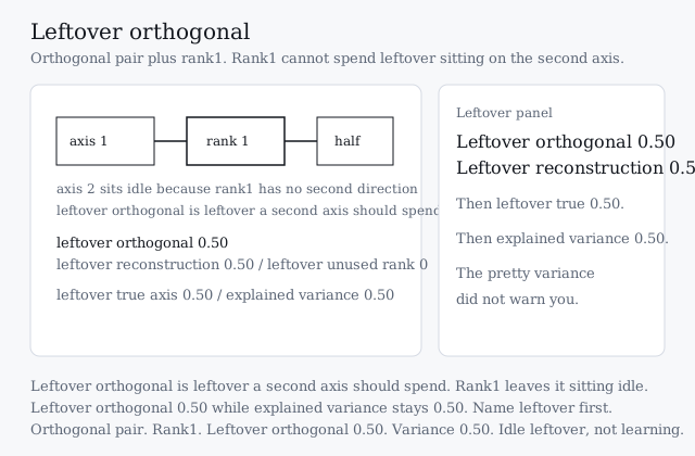
Switch the intro lab to orthogonal leftover and rank1. Leftover orthogonal rises to 0.50. Leftover reconstruction rises to 0.50. Leftover unused rank stays 0. Leftover on true axis is 0.50. Explained variance is 0.50. Leftover orthogonal. The pretty variance did not warn you. Idle orthogonal leftover is leftover, not learning.

Home leftover orthogonal 0 is modest leftover because the home pair is aligned. Leftover orthogonal 0.50 is leftover unused axis.

Name leftover orthogonal first, then leftover reconstruction, then leftover on true axis, then explained variance.

import numpy as np

# Home aligned leftover: leftover reconstruction spent on a direction.
home_a = np.array([1.0, 0.2])
home_b = np.array([0.9, 0.25])
# Orthogonal leftover: leftover orthogonal sits because rank1 cannot spend it.
orth_a = np.array([1.0, 0.0])
orth_b = np.array([0.0, 1.0])

def leftover_orthogonal(a, b):
    proj = (a @ b) / (a @ a) * a
    residual = b - proj
    return float(np.linalg.norm(residual) / (np.linalg.norm(b) + 1e-12))

Home leftover reconstruction 0.13 is leftover the aligned rank1 still has to spend. Leftover orthogonal 0.50 is leftover unused axis.

Why Extra Unused Rank Leaves Leftover Unused Rank

A second axis can spend leftover orthogonal. On an aligned pair it can also leave leftover unused rank: extra axes cover leftover rank1 would have spent locally.

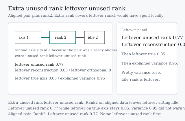
Switch the intro lab to aligned leftover and rank2. Leftover unused rank rises to 0.77. Leftover reconstruction drops to 0.05. Leftover on true axis drops to 0.05. Leftover orthogonal stays 0. Explained variance is 0.95. Extra unused rank leftover unused rank. The pretty variance did not warn you. Idle extra rank is leftover, not learning.

Home leftover unused rank 0.11 is modest leftover. Extra unused rank leftover unused rank 0.77 is leftover unused axis capacity.

Name leftover unused rank first, then leftover reconstruction, then leftover on true axis, then explained variance.

The leftover lab below starts leftover present on the rank1 path. Leftover orthogonal is 0.50 while explained variance stays 0.50. Rank2 leftover orthogonal is 0.09. Leftover absent leftover orthogonal is 0.

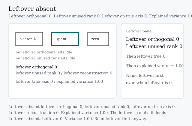
Leftover absent leftover orthogonal 0, leftover unused rank 0, leftover on true axis 0, leftover reconstruction 0. Explained variance 1.00. Name leftover first even when leftover is already 0.

Rank2 leftover spend on an orthogonal pair: leftover orthogonal 0.09, leftover unused rank 0.15, leftover on true axis 0.09, leftover reconstruction 0.09, explained variance 0.91. A second axis spends leftover orthogonal. Leftover unused rank 0.15 is leftover the extra capacity still has to spend.

The Language of Data: Scalars, Vectors, Matrices, and Tensors

In deep learning, data is leftover sitting in linear-algebra objects. Understanding these is leftover a practitioner has to spend.

• Scalar: A single number (e.g., $a \in \mathbb{R}$). A scalar recipe cannot spend leftover reconstruction.
• Vector: An ordered array of numbers. We denote a vector in $\mathbb{R}^n$ as a column vector $\mathbf{x} = [x_1, x_2, \dots, x_n]^T$. Vectors can represent a point in an n-dimensional space or a set of features for a single data sample. Home leftover reconstruction 0.13 lives on a pair of vectors.
• Matrix: A 2D array of numbers, denoted $\mathbf{A} \in \mathbb{R}^{m \times n}$. A matrix can represent an entire dataset, where m is the number of samples and n is the number of features, or it can represent a linear transformation that spends leftover on columns.
• Tensor: A generalization of these objects to more than two dimensions. For example, a color image can be represented as a 3D tensor of shape (height, width, channels). Leftover reconstruction still has a direction even when the object is a tensor.

These are not merely abstract concepts; they correspond directly to the ndarray in NumPy or Tensor in PyTorch/TensorFlow, the primary data structures used in deep learning frameworks.

Core Operations: Dot Products and Matrix Multiplication

The operations performed within neural networks are leftover spend built on elementary linear algebra.

• Dot Product: The dot product between two vectors $\mathbf{x}, \mathbf{y} \in \mathbb{R}^n$ is defined as $\mathbf{x}^T \mathbf{y} = \sum_{i=1}^n x_i y_i$. Geometrically, it relates to the projection of one vector onto another and can be used to compute the angle between them: $\mathbf{x}^T \mathbf{y} = \|\mathbf{x}\|_2 \|\mathbf{y}\|_2 \cos \theta$. Home leftover reconstruction 0.13 is leftover after that score is spent on an aligned pair. Leftover orthogonal 0.50 is leftover when the cosine is near 0.
• Matrix-Vector Product: The product of a matrix $\mathbf{A} \in \mathbb{R}^{m \times n}$ and a vector $\mathbf{x} \in \mathbb{R}^n$ results in a vector $\mathbf{y} \in \mathbb{R}^m$. This operation can be viewed as a linear combination of the columns of A, where the coefficients are the elements of x. Rank1 leftover spend is one column. Rank2 leftover spend is two columns.
• Matrix-Matrix Product: The product of two matrices $\mathbf{A} \in \mathbb{R}^{m \times n}$ and $\mathbf{B} \in \mathbb{R}^{n \times p}$ results in a matrix $\mathbf{C} \in \mathbb{R}^{m \times p}$. This operation corresponds to the composition of two linear transformations. A forward pass through a fully connected layer of a neural network is precisely a matrix-vector product ($\mathbf{W}\mathbf{x}$) followed by the addition of a bias vector (+b). Leftover reconstruction after $\mathbf{W}\mathbf{x}$ is leftover the next layer should spend.

Decomposing Matrices: Eigendecomposition and SVD

Matrix decompositions name leftover axes of a transformation.

• Eigendecomposition: For a square matrix $\mathbf{A} \in \mathbb{R}^{n \times n}$, an eigenvector $\mathbf{v}$ is a non-zero vector that does not change direction when transformed by A, only its scale changes. This relationship is captured by the equation:

  $$\mathbf{A}\mathbf{v} = \lambda \mathbf{v}$$

  Here, $\lambda$ is the scalar eigenvalue corresponding to the eigenvector $\mathbf{v}$. Eigenvectors represent the principal axes of the transformation, and eigenvalues represent the scaling factor along these axes. If a matrix A has n linearly independent eigenvectors, it can be decomposed into:

  $$\mathbf{A} = \mathbf{V} \Lambda \mathbf{V}^{-1}$$

  where V is the matrix whose columns are the eigenvectors of A, and $\Lambda$ is a diagonal matrix containing the corresponding eigenvalues. For real symmetric matrices, the eigenvectors are orthogonal, so $\mathbf{V}^{-1} = \mathbf{V}^T$. Leftover orthogonal 0.50 is leftover sitting on an unused eigenvector when rank is 1.

• Singular Value Decomposition (SVD): SVD is a more general decomposition that applies to any matrix $\mathbf{A} \in \mathbb{R}^{m \times n}$. It factors A into three matrices:

  $$\mathbf{A} = \mathbf{U} \Sigma \mathbf{V}^T$$

  where:

  • $\mathbf{U} \in \mathbb{R}^{m \times m}$ is an orthogonal matrix whose columns are the left-singular vectors.
  • $\mathbf{V} \in \mathbb{R}^{n \times n}$ is an orthogonal matrix whose columns are the right-singular vectors.
  • $\Sigma \in \mathbb{R}^{m \times n}$ is a diagonal matrix containing the singular values.

  The right-singular vectors of A are the eigenvectors of $\mathbf{A}^T\mathbf{A}$, and the left-singular vectors are the eigenvectors of $\mathbf{A}\mathbf{A}^T$. The non-zero singular values are the square roots of the non-zero eigenvalues of both $\mathbf{A}^T\mathbf{A}$ and $\mathbf{A}\mathbf{A}^T$. Extra unused rank leftover unused rank 0.77 is leftover sitting in a trailing singular value the aligned pair did not need.

Application: Principal Component Analysis (PCA)

PCA is leftover reconstruction spent as a lower-dimensional representation that preserves as much of the original variance as possible. Home leftover reconstruction 0.13 is leftover after rank1 on aligned data. Leftover orthogonal 0.50 is leftover after rank1 on an orthogonal pair.

Given a dataset represented by a matrix $\mathbf{X} \in \mathbb{R}^{m \times n}$ (where m is the number of samples and n is the number of features), and assuming the data is centered (mean of each feature is zero), PCA finds a new set of orthogonal axes, called principal components, that align with the directions of maximum variance in the data.

Mathematical Formulation: The problem can be formulated as finding a projection matrix W that maximizes the variance of the projected data XW. The solution is that the columns of W are the eigenvectors of the covariance matrix of the data, $\mathbf{C} = \frac{1}{m-1} \mathbf{X}^T \mathbf{X}$, corresponding to the largest eigenvalues. Leftover on the true axis 0.09 is leftover the home rank1 still has after that spend.

PCA via SVD: In practice, PCA is often computed using SVD because it is more numerically stable. The SVD of the centered data matrix X is $\mathbf{X} = \mathbf{U} \Sigma \mathbf{V}^T$. The principal components are the columns of V (the right-singular vectors of X), and the variance explained by each component is proportional to the square of the corresponding singular value in $\Sigma$. Name leftover reconstruction first, then leftover unused rank, then leftover on true axis, then explained variance.

This connection between classical linear algebra and deep learning is leftover a linear autoencoder should spend. An autoencoder is a neural network trained to reconstruct its input, typically through a low-dimensional bottleneck layer. If an autoencoder has a single hidden layer with a linear activation function and is trained to minimize the mean squared reconstruction error, it learns to project the data onto the same principal subspace identified by PCA. Leftover reconstruction 0.13 is leftover that bottleneck still has to spend on the home aligned rank1.

Failure Mode

Quote explained variance 0.50 on an orthogonal pair, then skip leftover orthogonal 0.50. Quote explained variance 0.95 after extra unused rank, then skip leftover unused rank 0.77. Home leftover reconstruction 0.13 is the number to read first. Explained variance 0.91 still looks fine.

Path Forward

Leftover orthogonal is the seed of the next lesson. What rank1 cannot spend, a second axis can. Probability leftover and information leftover are how the next lesson spends leftover reconstruction.

References

1. Goodfellow, I., Bengio, Y., and Courville, A. (2016). Deep Learning. MIT Press. Chapters 2 and 13.
2. Strang, G. (2016). Introduction to Linear Algebra. Wellesley-Cambridge Press.
3. Trefethen, L. N., and Bau, D. (1997). Numerical Linear Algebra. SIAM.
4. Pearson, K. (1901). On lines and planes of closest fit to systems of points in space. Philosophical Magazine.