Introduction to Deep Learning: Leftover Representation, Then Accuracy

Deep learning spends leftover representation that a rule list cannot spend. A perceptron spends leftover on linearly separable data. Leftover xor is what a hidden layer should spend. Extra unused depth leftover unused depth. Leftover on the true class remains after the forward pass. Home still names leftover first, then the pretty accuracy.

The key question is:

After the forward pass, what leftover representation remains, and did leftover xor sit idle because the separator was a line or leftover unused depth sit idle because the hidden layer was extra?

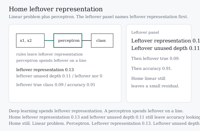
Home still in the lab below is leftover representation: leftover representation 0.13, leftover unused depth 0.11, leftover xor 0, leftover on true class 0.09. Accuracy still looks fine at 0.91.

A rule list treats knowledge as leftover already spent as hard-coded facts. Face leftover, speech leftover, and pixel leftover sit idle because nobody wrote the rule. Representation leftover is leftover a hierarchy of features should spend: edges, then parts, then the concept.

A perceptron spends leftover representation on a line. Weighted inputs plus a bias write a score. A step function spends leftover on one side of that line. Shared leftover spend is reused on every example.

The core update is:

$$\hat{y} = f(\mathbf{w}^{T} \mathbf{x} + b)$$

where $\mathbf{x}$ is available at prediction time, $\mathbf{w}$ is leftover importance, $b$ shifts the line, and $f$ is the step. Home leftover representation 0.13 means the linear still left a small residual to spend. Leftover unused depth 0.11 is modest leftover. Read leftover first.

From Line to Hidden Layer

After the forward pass, a hidden layer spends leftover xor. A perceptron spends leftover representation locally on a line. Extra unused depth leftover unused depth sits idle in hidden units the linear problem did not need.

Typical stack:

1. Score $$z = \mathbf{w}^{T} \mathbf{x} + b$$
2. Step $$\hat{y} = 1 \text{ if } z \ge 0 \text{ else } 0$$
3. Leftover xor $$\text{leftover xor sits when one line cannot spend XOR}$$

Home leftover unused depth 0.11 is the honest leftover after a linear problem and a perceptron. Leftover xor 0.50 is leftover sitting idle when the separator is a line on XOR.

Use the lab above as the mental model for the rest of the lesson. On the home linear perceptron, leftover representation is 0.13 and leftover unused depth is 0.11. Accuracy still looks fine at 0.91.

Why Leftover Xor Sits Idle on a Line

XOR asks a line to separate (0,0) and (1,1) from (0,1) and (1,0). That leftover cannot be spent by one hyperplane. Leftover xor is leftover a hidden layer should spend.

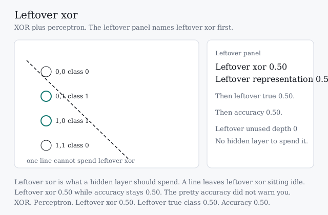
Switch the intro lab to XOR leftover and perceptron. Leftover xor rises to 0.50. Leftover representation rises to 0.50. Leftover unused depth stays 0. Leftover on true class is 0.50. Accuracy is 0.50. Leftover xor. The pretty accuracy did not warn you. Idle XOR leftover is leftover, not learning.

Home leftover xor 0 is modest leftover because the home problem is linear. Leftover xor 0.50 is leftover unused separator.

Name leftover xor first, then leftover representation, then leftover on true class, then accuracy.

import numpy as np

# Home linear leftover: leftover representation spent on a line.
home_x = np.array([[0.0, 0.0], [1.0, 1.0]])
home_y = np.array([0, 1])
# XOR leftover: leftover xor sits because one line cannot spend it.
xor_x = np.array([[0.0, 0.0], [0.0, 1.0], [1.0, 0.0], [1.0, 1.0]])
xor_y = np.array([0, 1, 1, 0])

def perceptron_score(x, w, b):
    return x @ w + b

Home leftover representation 0.13 is leftover the linear perceptron still has to spend. Leftover xor 0.50 is leftover unused separator.

Why Extra Unused Depth Leaves Leftover Unused Depth

A hidden layer can spend leftover xor. On a linear problem it can also leave leftover unused depth: extra units cover leftover the perceptron would have spent locally.

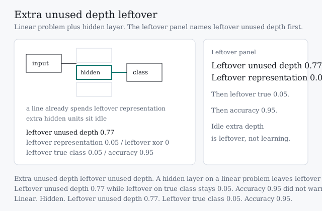
Switch the intro lab to linear leftover and hidden. Leftover unused depth rises to 0.77. Leftover representation drops to 0.05. Leftover on true class drops to 0.05. Leftover xor stays 0. Accuracy is 0.95. Extra unused depth leftover unused depth. The pretty accuracy did not warn you. Idle extra depth is leftover, not learning.

Home leftover unused depth 0.11 is modest leftover. Extra unused depth leftover unused depth 0.77 is leftover unused hidden capacity.

Name leftover unused depth first, then leftover representation, then leftover on true class, then accuracy.

The leftover lab below starts leftover present on the linear path. Leftover xor is 0.50 while accuracy stays 0.50. Hidden leftover xor is 0.09. Leftover absent leftover xor is 0.

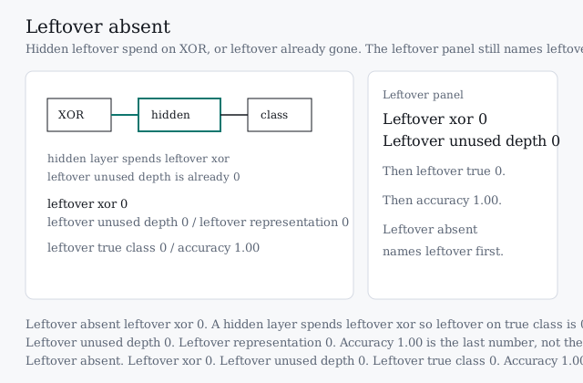
Leftover absent leftover xor 0, leftover unused depth 0, leftover on true class 0, leftover representation 0. Accuracy 1.00. Name leftover first even when leftover is already 0.

Hidden leftover spend on XOR: leftover xor 0.09, leftover unused depth 0.15, leftover on true class 0.09, leftover representation 0.09, accuracy 0.91. A hidden layer spends leftover xor. Leftover unused depth 0.15 is leftover the extra capacity still has to spend.

The perceptron learning rule is leftover-driven correction. If a positive example is leftover miss, the weights spend leftover toward the true class. If a negative example is leftover miss, the weights spend leftover the other way. Home leftover on true class 0.09 is leftover the linear still has after that spend. Leftover xor 0.50 is leftover the rule cannot spend because the points are not on a line.

Failure Mode

Quote accuracy 0.50 on XOR, then skip leftover xor 0.50. Quote accuracy 0.95 after extra unused depth, then skip leftover unused depth 0.77. Home leftover representation 0.13 is the number to read first. Accuracy 0.91 still looks fine.

Path Forward

Leftover xor is the seed of the next lesson. What one perceptron cannot spend, a hidden layer can. Multi-layer leftover composition is how depth spends leftover representation.

References

1. Goodfellow, I., Bengio, Y., and Courville, A. (2016). Deep Learning. MIT Press.
2. Rosenblatt, F. (1958). The perceptron: A probabilistic model for information storage and organization in the brain. Psychological Review.
3. Minsky, M. L., and Papert, S. A. (1969). Perceptrons: An introduction to computational geometry. MIT Press.
4. McCulloch, W. S., and Pitts, W. (1943). A logical calculus of the ideas immanent in nervous activity. The Bulletin of Mathematical Biophysics.